VGG

#

This is a Pytorch implementation of the Very Deep Convolutional Networks for Large-Scale Image Recognition paper by Karen Simonyan and Andrew Zisserman.

The VGG paper was unique for their time, as it proved the importance of depth in image classification. Unlike their predecessors, VGG models utilize simple filters and a repetitive structure. In return for its simplicity, VGG has a far greater depth, the deepest variation in the paper having 19 layers, which was a lot for its time.

Accompanying blog post

import torch
import torch.nn as nn
from torchinfo import summary

#

Model Architecture

#

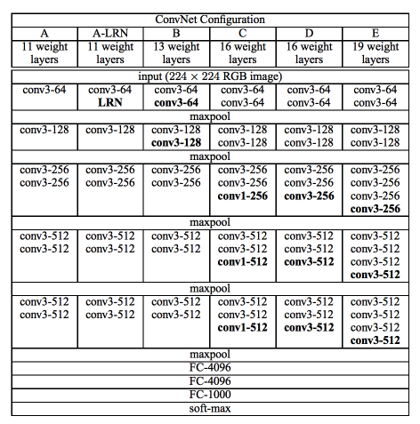
There are 6 VGG papers introduced in the paper, the primary ones being VGG11, VGG13, VGG16, and VGG19.

The CONFIGURATION dictionary contains nested lists for each model. Each array in the list represents a single block, and each entry in the array represents the type of layer:

If the layer is represented by the number $n$, it is a $3 \times 3$ convolution with $n$ filters.
If the layer is represented by the string ‘M’, it is a Maxpool layer.

CONFIGURATION = {
    "VGG11": [
        [64,'M'],
        [128,'M'],
        [256,256,'M'],
        [512,512,'M'],
        [512,512,'M']
    ],
    "VGG13": [
        [64,64,'M'],
        [128,128,'M'],
        [256,256,'M'],
        [512,512,'M'],
        [512,512,'M']
    ],
    "VGG16": [
        [64,64,'M'],
        [128,128,'M'],
        [256,256,256,'M'],
        [512,512,512,'M'],
        [512,512,512,'M']
    ],
    "VGG19": [
        [64,64,'M'],
        [128,128,'M'],
        [256,256,256,256,'M'],
        [512,512,512,512,'M'],
        [512,512,512,512,'M']
    ]
}

#

VGG Model

#

This is the main part of the VGG model.

#

class VGGModel(nn.Module):

#

Parameters

architecture_name: the name of the VGG model, like “VGG16” or “VGG19”
input_width: the width of the input image
num_output: the number of classes

    def __init__(self, architecture_name, input_width, num_output):

#

Generate the Pytorch model from the given nested list.

        super(VGGModel, self).__init__()
        self.architecture = self.create_architecture(CONFIGURATION.get(architecture_name), input_width, num_output)

#

        self.block1 = self.architecture[0]
        self.block2 = self.architecture[1]
        self.block3 = self.architecture[2]
        self.block4 = self.architecture[3]
        self.block5 = self.architecture[4]
        self.block6 = self.architecture[5]
        self.flat = nn.Flatten()

#

Propagate through the network.

x has the input dimensions (batch_size, input_channels, image_height, image_width)

    def forward(self,x):

#

Blocks 1 ~ 5

        z = self.block1(x)
        z = self.block2(z)
        z = self.block3(z)
        z = self.block4(z)
        z = self.block5(z)

#

Flatten layer to connect the feature map to a FC layer.

        z = self.flat(z)

#

Final layers to produce the image classification prediction.

        z = self.block6(z)

#

        return z

#

Parameters

architecture: 2D list of int and string that represent layers
num_outputs: Number of output classes at the end of the network

Returns

blocks_list: List of PyTorch NN sequences, each representing one block

    def create_architecture(self, architecture, input_width, num_outputs):

#

Store all blocks in blocks_list to be returned.

        blocks_list = []

#

Assume the input image has 3 channels (RGB).

        num_next_input_channels = 3

#

Create convolutional blocks. num_next_input_channels keeps track of the number of channels to be input into the next block.

        
        for block in architecture:
            num_next_input_channels, layers = self.create_block(block, num_next_input_channels)
            blocks_list.append(layers)

#

        blocks_list.append(

#

Create the final block.

            nn.Sequential(

#

A Fully Connected layer with the dimensions of $(512 \cdot (\frac{input width}{32})^2, 1000)$.

#

There are 5 MaxPool layers in the network, so the input_width entered in the beginning is halved five times (so divided by 32 overall). The final layer in the 5th block of VGG uses 512 filters, meaning that the output result of the 5th block would be (batch_size, 512, input_height // 32, input_width // 32). We are assuming that the input images are squares.

#

Once the result passes through the nn.Flatten() layer, the dimensions would be $(batch size, 512 \cdot (\frac{input width}{32})^2)$. The FC layer contains 4096 neurons, so the dimensions of the FC layer would be $(512 \cdot (\frac{input width}{32})^2, 1000)$.

                        nn.Linear(512*int(input_width / 32)**2, 4096), # 32 = 2**5

#

ReLU

                        nn.ReLU(),

#

The output of the previous FC layer is (batch_size, 4096). This FC layer also has 4096 neurons, so its dimension is $(4096,4096)$

                        nn.Linear(4096,4096),

#

ReLU

                        nn.ReLU(),

#

The final FC layer outputs (batch_size, num_outputs).

                        nn.Linear(4096, num_outputs),

#

Softmax

                        nn.Softmax(dim=1))
        )


        return blocks_list

#

Create a singular block.

Parameters

block: 1D list of int and string of block, where each entry is either the number of filters in the Conv2d layer or a str indication of MaxPool2d

Returns

num_channels: output number of channels of the convolutional block
layers: nn.Sequential for a singular block in VGG

    def create_block(self, block, num_next_input_channels):

#

Keep track of number of channels passed between Conv2d layers.

        layers_list = []
        num_channels = num_next_input_channels

#

The original VGG paper follows Conv2d -> ReLU for each conv layer, but BatchNorm was added to handle overfitting.

The paper explicitly mentions that it only uses convolutional filters with kernel size $3 \times 3$. The paper utilizes “same” convolutions (convolutions that do not change the output width and height). From the following equation for output dimension,

$$n_{out} = \lfloor \frac{n_{in} + 2p - k}{s} \rfloor + 1$$

we get that the stride and padding are both 1.

        for layer in block:
                if isinstance(layer, int):
                    layers_list += [
                        nn.Conv2d(in_channels=num_channels, out_channels=layer, kernel_size=(3,3), stride=(1,1), padding=(1,1)),
                        nn.BatchNorm2d(layer), 
                        nn.ReLU()
                    ]

#

On the other hand, the MaxPool layers halve the input dimensioins, so the stride is 2.

                    num_channels = layer
                else:
                    layers_list += [
                        nn.MaxPool2d(kernel_size=2, stride=2)
                    ]

#

Sample tensor simulating one training instance from ImageNet

        layers = nn.Sequential(*layers_list)
        return num_channels, layers


if __name__ == "__main__":
    testing = VGGModel("VGG19", 224, 1000)
    t1 = torch.randn(1,3,224,224)

#

Print result: (1,1000)

    print(testing(t1).size())

#