MobileNetV2
This is a Pytorch implementation of the MobileNetV2: Inverted Residuals and Linear Bottlenecks paper.
MobileNetV2, like its predecessor MobileNetV1, is designed for mobile resource-constrained devices. The key improvement is the the addition of inverted residual blocks and linear bottlenecks. Both inverted residual block and linear bottleneck concepts stem from residual blocks from ResNet.
The inclusion of the two concepts help make MobileNetV2 computationally efficient while having higher accuracy than MobileNetV1. MobileNetV2 is suited for real-time applications and mobile platforms.
It is strongly to be familiar with Residual Learning before studying MobileNetV2.
Depthwise Separable Convolutions

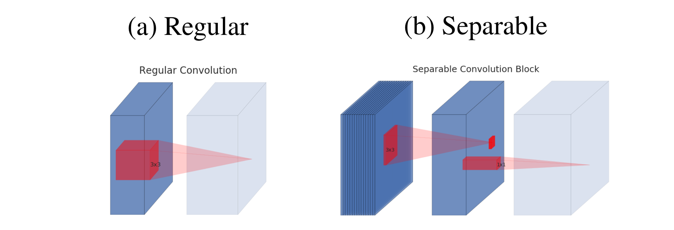
Depthwise separable convolutions are specific convolution types used in inverted residual learning. Depthwise separable convolutions use a two-step process of depthwise convolution and pointwise convolution.
While standard convolutions take an (batch_size, channel_num, height, width) and
apply filter_num convolutional filters of (channel_num, filter_height, filter_width)
to produce an output of (batch_size, filter_num, height, width). The computationl cost is
height*width*channel_num*filter_num*filter_height*filter_width.
On the other hand, depthwise convolutions use filter_num convolutional filters of
(1, filter_height, filter_width). The filters are applied to each individual
feature map and are combined back together to return an output of (batch_size, channel_num, height, width).
Then, the pointwise convolution builds new features by computing linear combinations
of the feature spaces by applying filter_num convolution filters of (channel_num, filter_num, 1, 1).
Thus, the computational cost of depthwise separable convolutions is height*width*channel_num*(filter_height+filter_width + filter_num),
indicating a reduction of computational cost.
Linear Bottlenecks

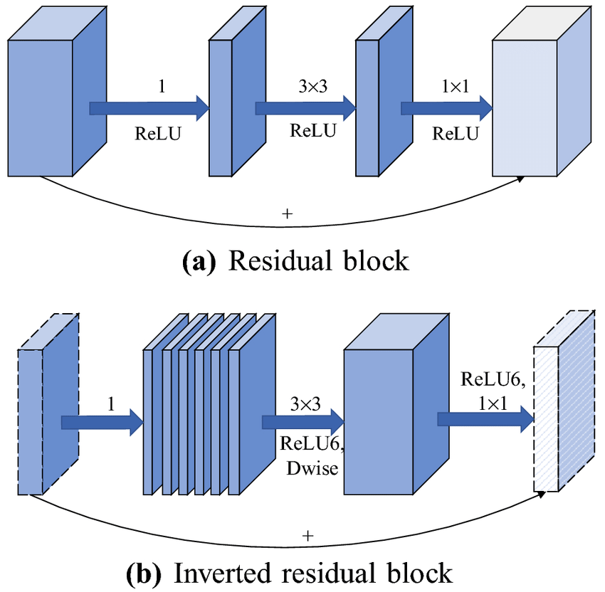
Much like the ResNet linear bottlenecks, MobileNetV2 linear bottlenecks use two \(1 \times 1\) convolutions and one \(3 \times 3\) convolution. The difference is that MobileNetV2 uses \(1 \times 1\) expansion layer, \(3 \times 3\) depthwise convolution layer, and a \(1 \times 1\) projection layer.
While a normal residual block bottleneck has a high number of input channels and follows a wide -> narrow -> wide approach (compression, convolution, expansion), the inverted residual block bottleneck has fewer number of input channels and follows a narrow -> wide -> narrow approach (expansion, depthwise, compression) approach.
import torch
import torch.nn as nn
from torchinfo import summaryInverted Residual Block
class InvertedResidualBlock(nn.Module):Parameters
input_channels: input number of channels
output_channels: output number of channels
expansion: the expansion ratio for the number of channels
stride: the stride length of the depthwise convolution. Stride is 1 when repeating the same
inverted residual block and 2 when downsampling is used.
The shortcut connection will use the same stride to keep the dimensions the same.
    def __init__(self, input_channels, output_channels, expansion, stride=1):
super(InvertedResidualBlock, self).__init__() self.block = nn.Sequential((Expansion) \(1 \times 1\) convolutional layer to map channel length to input_channels*expansion.
            nn.Conv2d(in_channels=input_channels,
                      out_channels=input_channels*expansion,
                      kernel_size=1,
                      stride=1,
                      padding=0,
bias=False),First batch normalization
nn.BatchNorm2d(input_channels*expansion),ReLU
nn.ReLU(),(Depthwise) \(3 \times 3\) convolutional layer to learn features
            nn.Conv2d(in_channels=input_channels*expansion,
                      out_channels=input_channels*expansion,
                      kernel_size=3,
                      stride=stride,
                      padding=1,
                      groups=input_channels*expansion,
bias=False),Second batch normalization
nn.BatchNorm2d(input_channels*expansion),ReLU
nn.ReLU(),(Compression) \(1 \times 1\) convolutional layer to compress the number of channels to output_channels
            nn.Conv2d(in_channels=input_channels*expansion,
                      out_channels=output_channels,
                      kernel_size=1,
                      stride=1,
                      padding=0,
bias=False),Final batch normalization
            nn.BatchNorm2d(output_channels)
)Final ReLU
        self.relu = nn.ReLU()

if stride != 1 or input_channels != output_channels:If input and output are different dimensions (stride is not 1), W_i from the shortcut
connection maps the number of channels in x (input_channels) to the output_channels
using a \(1 \times 1\) convolution to keep the width and height the same.
Additionally, if the input_channels is not equal to output_channels,
then use a \(1 \times 1\) convolution to equalize number of channels.
            self.shortcut = nn.Sequential(
                nn.Conv2d(in_channels=input_channels,
                          out_channels=output_channels,
                          kernel_size=1,
                          stride=stride,
                          padding=0,
                          bias=False),
                nn.BatchNorm2d(output_channels)
            )
        else:
self.shortcut = nn.Sequential() def forward(self, x):
z = self.block(x)
z += self.shortcut(x)
z = self.relu(z)
return zMobileNetV2 Model
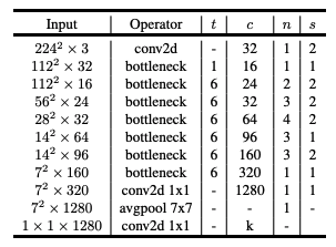
class MobileNetV2(nn.Module):MobileNetV2 configuration mentioned in the paper. Each list represents a bottleneck layer,
and the list contains:
[t (expansion), c (output channels), n (repetition number), s (stride)].
    configuration = [
        [1, 16, 1, 1],
        [6, 24, 2, 2],
        [6, 32, 3, 2],
        [6, 64, 4, 2],
        [6, 96, 3, 1],
        [6, 160, 3, 2],
        [6, 320, 1, 1]
]Parameters
input_width: the width of the input image
output_num: the number of classes
input_channels: the number input channels (3 for RGB images)
def __init__(self, input_width, output_num, input_channels=3): super(MobileNetV2, self).__init__()Keep track of the number of feature maps throughout the network
self.current_channels = 32 self.preliminary = nn.Sequential(
nn.Conv2d(in_channels=input_channels,
out_channels=self.current_channels,
kernel_size=3,
stride=2,
padding=1,
bias=False),
nn.BatchNorm2d(self.current_channels),
nn.ReLU()
) self.layer1 = self.make_layer(self.configuration[0])
self.layer2 = self.make_layer(self.configuration[1])
self.layer3 = self.make_layer(self.configuration[2])
self.layer4 = self.make_layer(self.configuration[3])
self.layer5 = self.make_layer(self.configuration[4])
self.layer6 = self.make_layer(self.configuration[5])
self.layer7 = self.make_layer(self.configuration[6])Final layer
Consists of Conv2d -> Flatten -> FC -> Softmax Since the input was downsampled 5 times throughout the network, the input width/height at the end is halved 5 times.
        self.final = nn.Sequential(
            nn.Conv2d(in_channels=self.current_channels,
                      out_channels=1280,
                      kernel_size=1,
                      stride=1,
                      padding=0,
                      bias=False),
            nn.Flatten(),
            nn.Linear(in_features=1280*int(input_width/(2**5))**2, out_features=output_num),
            nn.Softmax(dim=1)
)Propagate
    def forward(self,x):
        z = self.preliminary(x)

        z = self.layer1(z)
        z = self.layer2(z)
        z = self.layer3(z)
        z = self.layer4(z)
        z = self.layer5(z)
        z = self.layer6(z)
        z = self.layer7(z)

        z = self.final(z)
return zCreate layer of Inverted Residual Blocks
def make_layer(self, layer_cofig):Create a layer.
Parameters
layer_config: parameter configuration
Returns
nn.Sequential(*layers): Sequence of layers in the whole Inverted Residual Block layer
        expansion, output_channels, repetition_num, stride = layer_cofig

        layers = []
        for _ in range(repetition_num):
            layers.append(InvertedResidualBlock(self.current_channels, output_channels, expansion, stride=stride))
            self.current_channels = output_channels
            stride = 1
return nn.Sequential(*layers)Tensor Test
if __name__ == "__main__":Sample tensor simulating one training instance from ImageNet
img = torch.randn(1,3,224,224)MobileNetV2
test_model = MobileNetV2(224,1000)Size output: (1,1000)
print(test_model(img).size())
