EfficientNet

#

This is a Pytorch implementation of the EfficientNet: Rethinking Model Scaling for Convolutional Neural Networks paper.

Unlike ResNet, MobileNetV2, or some other models, EfficientNet does not introduce a completely new architecture concept. Instead, it introduces the idea of compound scaling, stochastic depth, and a base model, EfficientNet, to test the new scaling method.

The EfficientNet utilizes Inverted Residual Blocks from MobileNetV2, Squeeze-and-Efficient layers from SE-Net, so background knowledge on both are heavily recommended.

Scaling and Balancing

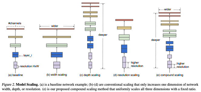
The authors argue that while scaling up depth, width, image resolution are common techniques to improve the model performance, previous papers use arbitrary scaling.

Depth is the most common method of scaling models. The VGG paper introduced the importance of depth, while ResNet and Densenet helped resolve the issue of training degradation.

Shallow networks generally use width scaling to capture features while being easy to train.

Scaling resolution is uncommon, but some networks GPipe utilize this to perform better. Resolution scaling is essentially increasing the width and height of the input images.

The empirical results of the paper indicate that a balance among width/depth/resolution can be achieved through compound scaling, which scales all three by a constant factor.

Compound Scaling

The idea behind compound scaling is to uniformly scale the depth, width, and resolution of the network in a principled manner. The authors introduce a compound coefficient, denoted as $\phi$, that controls the scaling factor for each dimension. By varying the value of $\phi$, the network can be scaled up or down while maintaining a balance among depth, width, and resolution.

The compound scaling is achieved by applying a set of predefined scaling rules. These rules specify how the depth, width, and resolution should be scaled based on the compound coefficient $\phi$. By following these rules, the network’s capacity is increased in a balanced way, ensuring that no individual dimension dominates the scaling process.

$$depth: d = \alpha^{\phi}$$
$$width: w = \beta^{\phi}$$
$$resolution: r = \gamma^{\phi}$$
such that $\alpha \dot \beta^2 \dot \gamma^2 \approx 2$ and $\alpha \geq 1, \beta \geq 1, \gamma \geq 1$.

For EfficientNetB0, the authors first fixed $\phi$ at 1 and performed a grid search for $\alpha, \beta, \gamma$ based on the equations above. The results showed that the best values are

$$\alpha = 1.2, \beta = 1.1, \gamma = 1.15.$$

The authors used this approach to minimize search cost, but it is technically possible to find the optimal $\alpha, \beta, \gamma$values using a larger model.

Stochastic Depth

Stochastic depth is essentially dropout for layers. For each mini-batch, some residual layers are completely dropped and only the residual skip connections are passed along.

This allows the network to train with a shorter effective depth, reducing the risk of overfitting and promoting regularization. By randomly dropping layers, stochastic depth provides a form of regularization similar to dropout but specifically tailored for residual networks.

Note: The authors of the paper use SiLU instead of ReLU.

Accompanying blog post

import torch
import torch.nn as nn
from torchinfo import summary

#

EfficientNetB0 Configuration

#

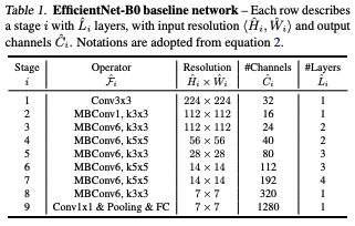
EfficientNet_B0 = [

#

EfficientNetB0 configuration mentioned in the paper. Each list represents a bottleneck layer, and the list contains:
[t (expansion), c (number of output channels), L (number of layers), k (kernel size), s (stride)].

    [1, 16, 1, 3, 1],
    [6, 24, 2, 3, 2],
    [6, 40, 2, 5, 2],
    [6, 80, 3, 3, 2],
    [6, 112, 3, 5, 1],
    [6, 192, 4, 5, 2],
    [6, 320, 1, 3, 1]
]

#

The phi value, resolution, and stochastic depth drop rate mentioned in the paper.

phi_values = (0, 224, 0.2)

#

Standard Convolutional Block

#

Standard convolutional block refactored due to high reuse in the model.

class ConvBlock(nn.Module):

#

Parameters

input_channels: input number of channels
output_channels: output number of channels
kernel_size: kernel size of the convolution filter
stride: the stride length of the convolution
padding: the padding of the convolution
groups: standard vs depthwise convolution

    def __init__(self, input_channels, output_channels, kernel_size, stride, padding, groups=1, bias=False):

#

        super(ConvBlock, self).__init__()

#

Convolutional layer (either standard or depthwise)

        self.conv = nn.Conv2d(input_channels, output_channels, kernel_size, stride, padding, groups=groups)

#

Batch normalization

        self.batch = nn.BatchNorm2d(output_channels)

#

SiLU

        self.silu = nn.SiLU()

#

    def forward(self,x):
        z = self.conv(x)
        z = self.batch(z)
        return self.silu(z)

#

Squeeze-and-Excitation Block

#

More details

class SE_Net(nn.Module):

#

    def __init__(self, input_channels, reduction_ratio):
        super(SE_Net,self).__init__()
        self.sequence = nn.Sequential(

#

1. Squeeze

            nn.AdaptiveAvgPool2d((1,1)),
            nn.Flatten(),

#

2. Excitation

            nn.Linear(input_channels, input_channels // reduction_ratio, bias=False),

#

SiLU instead of ReLU

            nn.SiLU(),
            nn.Linear(input_channels // reduction_ratio, input_channels),
            nn.Sigmoid(),
            nn.Unflatten(1, (input_channels,1,1))
        )

#

    def forward(self,x):
        z = self.sequence(x)

#

3. Rescale

        z = x*z
        return z

#

Inverted Residual Block

#

More details

class InvertedResidualBlock(nn.Module):

#

Parameters

input_channels: input number of channels
output_channels: output number of channels
kernel_size: kernel size of the convolution
stride: the stride length of the depthwise convolution. Stride is 1 when repeating the same inverted residual block and 2 when downsampling is used. The shortcut connection will use the same stride to keep the dimensions the same.
padding: padding of the convolution
expansion: the expansion ratio for the number of channels
reduction_ratio: reduction ratio for the SE-Net
survival_prob: survival probability for stochastic depth

    def __init__(self, input_channels, output_channels, kernel_size, stride, padding, expansion, reduction_ratio=4, survival_prob=0.5):

#

        super(InvertedResidualBlock, self).__init__()
        self.survival_prob = survival_prob

#

True if residual will be used (when input and output dimensions are the same)

        self.residual = input_channels == output_channels and stride == 1
        hidden_dim = input_channels*expansion
        self.expand = input_channels != hidden_dim

#

Expand number of channels by expansion amount

        if self.expand:
            self.expand_conv = ConvBlock(input_channels, hidden_dim, kernel_size=3, stride=1, padding=1)

#

Inverted Residual Block with SE-Net

        self.conv = nn.Sequential(
            ConvBlock(hidden_dim, hidden_dim, kernel_size, stride, padding, groups=hidden_dim),
            SE_Net(hidden_dim, input_channels // reduction_ratio),
            nn.Conv2d(hidden_dim, output_channels, 1, bias=False),
            nn.BatchNorm2d(output_channels)
        )

#

Propagate

    def forward(self,x):
        z = self.expand_conv(x) if self.expand else x

#

Apply stochastic depth when residual is used (in between a one layer of Inverted Residual Block)

        if self.residual:
            return self.stochastic_depth(self.conv(z))
        else:
            return self.conv(z)

#

Stochastic depth

    def stochastic_depth(self, x):

#

Do not use stochastic depth when training

        if not self.training:
            return x
        else:

#

Drop certain outputs by random according to survival probability

            binary_tensor = torch.rand(x.shape[0],1,1,1,device=x.device) < self.survival_prob
            return torch.div(x, self.survival_prob) * binary_tensor

#

EfficientNet

#

This is the main part of the EfficientNet model.

class EfficientNet(nn.Module):

#

Parameters

num_output: the number of classes

    def __init__(self, num_output):

#

        super(EfficientNet, self).__init__()

#

Extract $\alpha, \beta,$ and dropout_rate

        width_factor, depth_factor, dropout_rate = self.calculate_factors()
        last_channels = int(1280*width_factor)
        self.pool = nn.AdaptiveAvgPool2d((1,1))

#

Inverted Residual layers

        self.features = self.create_features(width_factor, depth_factor, last_channels)

#

Classifier layer

        self.classifier = nn.Sequential(
            nn.Dropout(dropout_rate),
            nn.Linear(last_channels, num_output)
        )

#

    def forward(self, x):
        z = self.pool(self.features(x))
        z = self.classifier(z.view(z.shape[0],-1))
        return z

#

Extract $\alpha, \beta, and$ drop rate

    def calculate_factors(self, alpha=1.2, beta=1.1):

#

Parameters

alpha: the depth scaling factor
beta: the width scaling factor

#

Calculate depth and width according to the compound scaling equation

        phi, resolution, drop_rate = phi_values
        depth_factor = alpha**phi
        width_factor = beta**phi
        return width_factor, depth_factor, drop_rate

#

Create Inverted Residual layers with SE-Net

    def create_features(self, width_factor, depth_factor, last_channels):

#

Parameters

width_factor: the depth scaling amount
depth_factor: the width scaling amount
last_channels: output number of feature maps at the end of the final layer

        channels = int(32*width_factor)
        features = [ConvBlock(3, channels, 3, stride=2, padding=1)]
        in_channels = channels

        for expand_ratio, channels, num_layers, kernel_size, stride in EfficientNet_B0:
            output_channels = 4*int(channels*width_factor/4)
            layer_num = int(num_layers*depth_factor)

            for layer in range(layer_num):
                features.append(InvertedResidualBlock(in_channels,
                                                      output_channels,
                                                      kernel_size=kernel_size,
                                                      stride=stride if layer == 0 else 1,
                                                      padding=kernel_size//2,
                                                      expansion=expand_ratio))
                in_channels = output_channels
        features.append(ConvBlock(in_channels, last_channels, kernel_size=1, stride=1, padding=0))
        return nn.Sequential(*features)

#

Tensor Test

if __name__ == "__main__":

#

Sample tensor simulating one training instance from ImageNet

    test = torch.rand(1,3,224,224)

#

EfficientNet

    model = EfficientNet(1000)

#

Size output: (1,1000)

    print(model(test).size())